Hybridization chain reaction

In this case study, we demonstrate how EQTK can be used to compute equilibrium concentrations of a large number of chemical species by considering initiated living polymerization.

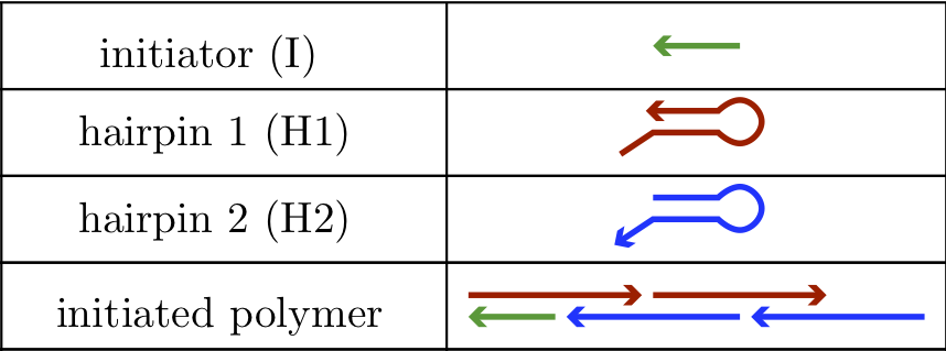
Dirks and Pierce (PNAS, 2004) published a living polymerization system constructed from single-stranded DNA molecules known as hybridization chain reaction, or HCR. The HCR system consists of three strand species in a dilute solution, initiator (I), hairpin 1 (H1), and hairpin 2 (H2), and is shown in the figure below. The sequences of the respective components are such that H1 and H2 minimally interact with each other in the absence of initiator, I. When I is introduced, H1 opens up, and can then bind H2. H2 in turn can bind another H1. This continues to form an initiated polymer of alternating H1 and H2 molecules.

Our goal in this case study is to compute the fraction of H1 and H2 molecules that are present in HCR polymers of each possible length \(n\). That is, we seek to understand how the H1 and H2 monomers are distributed among HCR polymers of various lengths. To be clear how we define polymer length, an HCR polymer of length \(5\) contains, in addition to the initiator strand, three H1 molecules and two H2 molecules.

To start the analysis, we import Numpy and EQTK, and additionally HoloViews for plotting, also setting some nice defaults for the plots.

import numpy as np
import eqtk

import holoviews as hv
hv.extension('bokeh')
hv.opts.defaults(
    hv.opts.Scatter(
        alpha=0.75,
        color=hv.Cycle(['#4c78a8', '#f58518', '#e45756']),
        fontsize=dict(labels=12, legend=8),
        height=350,
        padding=0.05,
        show_grid=True,
        size=5,
        toolbar="above",
        width=450,
    )
)

WARNING:param.main: pandas could not register all extension types imports failed with the following error: cannot import name 'ABCIndexClass' from 'pandas.core.dtypes.generic' (/Users/bois/opt/anaconda3/lib/python3.8/site-packages/pandas/core/dtypes/generic.py)

Chemical reactions and the stoichiometric matrix

The polymerization of HCR can be written as a set of chemical reactions with associated equilibrium constants. We write the reactions as dissociations. First, the initialization reaction,

\begin{align} \mathrm{I}\cdot\mathrm{H1} \rightleftharpoons \mathrm{I} + \mathrm{H1} ;\;\;K_I. \end{align}

After initialization, a polymer of even length (even number of total H1s and H2s, excluding initiator), can add an H1, and a polymer of odd length can add an H2.

\begin{align} &(n+1) \rightleftharpoons n + \mathrm{H1} ;\;\;K_1\;\;(n\text{ even}), \\[1em] &(n+1) \rightleftharpoons n + \mathrm{H2} ;\;\;K_2\;\;(n\text{ odd}). \end{align}

Note that by definition, \(n = 1\) corresponds to \(\mathrm{I}\cdot\mathrm{H1}\).

To codify this in a stoichiometric matrix \(\mathsf{N}\), we need to set a limit on how long the polymers can be. If we define this limit to be \(n_\mathrm{max}\), then we have a \(n_\mathrm{max} \times (n_\mathrm{max}+3)\) stoichiometric matrix, since each column corresponds to a chemical species. We use the first three columns for I, H1, and H2, respectively, and the remaining columns of for polymers of length 1, 2, 3, ….

We will write a function to generate a stoichiometric matrix as a Numpy array for a given \(n_\mathrm{max}\). It may help you understand how the function is used to construct the matrix if you look at the example with \(n_\mathrm{max} = 8\).

def hcr_N(n_max):
    """Generate a stoichiometric matrix for HCR with
    maximal polymer length `n_max`."""
    N = np.zeros((n_max, n_max + 3))
    N[0, 0:4] = np.array([1, 1, 0, -1])
    N[2::2, 1] = 1
    N[1::2, 2] = 1
    N[1:, 4:] -= np.eye(n_max - 1)
    N[1:, 3:-1] += np.eye(n_max - 1)

    return N

# Demonstrate with n_max = 0
hcr_N(8)

array([[ 1.,  1.,  0., -1.,  0.,  0.,  0.,  0.,  0.,  0.,  0.],
       [ 0.,  0.,  1.,  1., -1.,  0.,  0.,  0.,  0.,  0.,  0.],
       [ 0.,  1.,  0.,  0.,  1., -1.,  0.,  0.,  0.,  0.,  0.],
       [ 0.,  0.,  1.,  0.,  0.,  1., -1.,  0.,  0.,  0.,  0.],
       [ 0.,  1.,  0.,  0.,  0.,  0.,  1., -1.,  0.,  0.,  0.],
       [ 0.,  0.,  1.,  0.,  0.,  0.,  0.,  1., -1.,  0.,  0.],
       [ 0.,  1.,  0.,  0.,  0.,  0.,  0.,  0.,  1., -1.,  0.],
       [ 0.,  0.,  1.,  0.,  0.,  0.,  0.,  0.,  0.,  1., -1.]])

The first row is initialization of polymerization. The \(-1\) entry in the column with index 3 is the polymer of length 1, and the positive terms in the first two columns are for the initiator and H1.

The second row describes dissociation of a polymer of length 2, represented by the \(-1\) entry in the column with index 4. Upon dissociation, we are left with a polymer of length 1 (the +1 in column of index 3) and an H2 molecule (the +1 in column of index 2). The pattern continues as we grow longer polymers.

We will consider polymers up to length 2500.

n_max = 2500
N = hcr_N(n_max)

The equilibrium constants

We need to specify the three equilibrium constants, \(K_I\) for dissociation of I and H1, \(K_1\) for dissociation of H1 to the end of the polymer, and \(K_2\) for dissociation of H2 from the end of the polymer. We can compute the equilibrium constants from free energies of the respective chemical species and the number density of water, \(\rho_\mathrm{H_2O}\).

\begin{align} &K_I = \rho_\mathrm{H_2O}\,\exp\left[-\frac{G_\mathrm{I} + G_\mathrm{H1} - G_1}{k_BT}\right], \\[1em] &K_1 = \rho_\mathrm{H_2O}\,\exp\left[-\frac{G_2 + G_\mathrm{H1} - G_3}{k_BT}\right], \\[1em] &K_2 = \rho_\mathrm{H_2O}\,\exp\left[-\frac{G_1 + G_\mathrm{H2} - G_2}{k_BT}\right]. \\[1em] \end{align}

To compute the free energies, we can use the NUPACK web application.

# Free energies of HCR products, as calculated with NUPACK
# for DNA at 23 deg. C, values in kcal/mol
GI = -0.79
GH1 = -27.72
GH2 = -28.04
G1 = -41.52
G2 = -81.76
G3 = -121.97

When we compute the dissociation constants, we need to be mindful of units. First, we need to compute the thermal energy \(k_BT\), where \(k_B\) is the Boltzmann constant in units commensurate with those of the free energies. EQTK has a set of useful constants for unit conversion, so we can directly compute \(k_BT\) in the units that the NUPACK web application gave use for the free energies, kcal/mol.

# Thermal energy in units of kcal/mol
T = 23 + 273.15
kT = eqtk.constants.kB_kcal_per_mol_K * T

Next, we need to choose the units we wish to work with. Since HCR is usually done with species having concentrations in the micromolar range, we will choose to use dissociation constants with units of µM. To compute the density of water in units of µM, we can use eqtk.water_density().

# Number density of water in appropriate units
rho = eqtk.water_density(T=T, units='µM')

Finally, we can compute the equilibrium constants.

# Compute dissociation constants
KI = rho * np.exp(-(GH1 + GI - G2) / kT)
K1 = rho * np.exp(-(GH1 + G2 - G3) / kT)
K2 = rho * np.exp(-(GH2 + G1 - G2) / kT)

The reaction given by row zero of the stoichiometric matrix has equilibrium constant \(K_I\), that by row one has equilibrium constant \(K_2\), and that by row two had equilibrium constant \(K_1\). The rest of the rows alternate between \(K_2\) and \(K_1\). So, we can now set up our array of equilibrium constants for input into eqtk.solve().

# Equilibrium constants
K = np.zeros(len(N))
K[0] = KI
K[1::2] = K2
K[2::2] = K1

Initial concentrations

Finally, we need to specify the initial conditions of all chemical species. We will do the calculation with 1 µM each of H1 and H2, and vary the initiator concentration, considering [I]₀ = [0.01, 0.1, 1.0] µM.

# Initial concentrations of initiator
cI0 = [0.1, 0.03, 0.01]

# Build c0
c0 = np.zeros((3, n_max+3))
c0[:, 0] = cI0  # I
c0[:, 1] = 1.0  # H1
c0[:, 2] = 1.0  # H2

To make sure we understand how this is set up, we can look at the first eight columns.

c0[:, :8]

array([[0.1 , 1.  , 1.  , 0.  , 0.  , 0.  , 0.  , 0.  ],
       [0.03, 1.  , 1.  , 0.  , 0.  , 0.  , 0.  , 0.  ],
       [0.01, 1.  , 1.  , 0.  , 0.  , 0.  , 0.  , 0.  ]])

The column with index zero is the initiator concentration; the column with index one is the H1 concentration, and the column with index two is the H2 concentration. The rest of the columns are the initial concentration of HCR polymers, which we set to zero.

Each row of c0 represents a separate equilibrium calculation with the respective initial concentrations.

Solving for the concentrations

We now have the ingredients we need to solve for the concentrations of I, H1, H2, and all HCR polymers. We do this by calling eqtk.solve().

c = eqtk.solve(c0=c0, N=N, K=K, units='µM')

To investigate the output, we can look at the shape of the output array of concentrations.

c.shape

(3, 2503)

It has the same shape as the inputted c0, with each row corresponding to the equilibrium concentrations for the given initial concentrations.

Computing the mass-weighted polymer length distribution

Our next task is to compute fraction of H1 and H2 molecules that are present in HCR polymers of each length. Specifically, if \(n\) is the length of a polymer, this is

\begin{align} f_n = \frac{n c_n}{c_\mathrm{H1}^0 + c_\mathrm{H2}^0}, \end{align}

where \(c_n\) is the equilibrium concentration of HCR polymer of length \(n\), and \(c_\mathrm{H1}^0\) and \(c_\mathrm{H2}^0\) are respectively the total concentrations of H1 and H2.

n = np.arange(1, n_max + 1)
f = np.array([n * c[i, 3:] / (c0[i, 1] + c0[i, 2]) for i in range(3)])

Finally, we can plot the result.

pmf_plot = hv.Overlay(
    [
        hv.Scatter(
            data=(n, f[i]),
            kdims="n",
            vdims="mass-weighted probability",
            label=f"[I]₀ = {cI0[i]} µM",
        ).opts(logy=True, logx=True, ylim=(1e-5, 1e-1), fill_alpha=0.3)
        for i in range(3)
    ]
)

pmf_plot

Smaller initiator concentrations lead to longer polymers, as the curves shift rightward with decreasing initiator concentration. The curves also show an even-odd pattern, due to the fact that \(K_1\) and \(K_2\) are not equal.

A warning

HCR polymers can grow longer than a length of 2500, which we chose as our maximal allowed polymer length. For the initiator concentrations we considered here, negligible mass is contained in very long polymers. This is evident by the very steep drop off as \(n\) gets large in the mass-weighted probability mass function in the plot above.

If we choose \(n_\mathrm{max}\) to be too small, we would be missing all of the mass in longer polymers. Repeating the calculation with \(n_\mathrm{max} = 500\) shows the pathology.

n_max = 500
N = hcr_N(n_max)
K = K[:len(N)]
c0 = c0[:, :(n_max+3)]

c = eqtk.solve(c0=c0, N=N, K=K, units='µM')

n = np.arange(1, n_max + 1)
f = np.array([n * c[i, 3:] / (c0[i, 1] + c0[i, 2]) for i in range(3)])

# Construct plot
pmf_plot_500 = hv.Overlay(
    [
        hv.Scatter(
            data=(n, f[i]),
            kdims="n",
            vdims="mass-weighted probability",
        ).opts(logy=True, logx=True, ylim=(1e-5, 1e-1), marker="square", fill_alpha=0)
        for i in range(3)
    ]
)

pmf_plot * pmf_plot_500

The calculation with \(n_\mathrm{max} = 500\) is shown with squares. For larger initiator concentrations, we still accurately compute the mass-weighted probability mass function, but for the small initiator concentration, which gives longer polymers, the truncation error is substantial.

The lesson here is that EQTK will only consider the chemical species that are specifically given in the input, and no others.